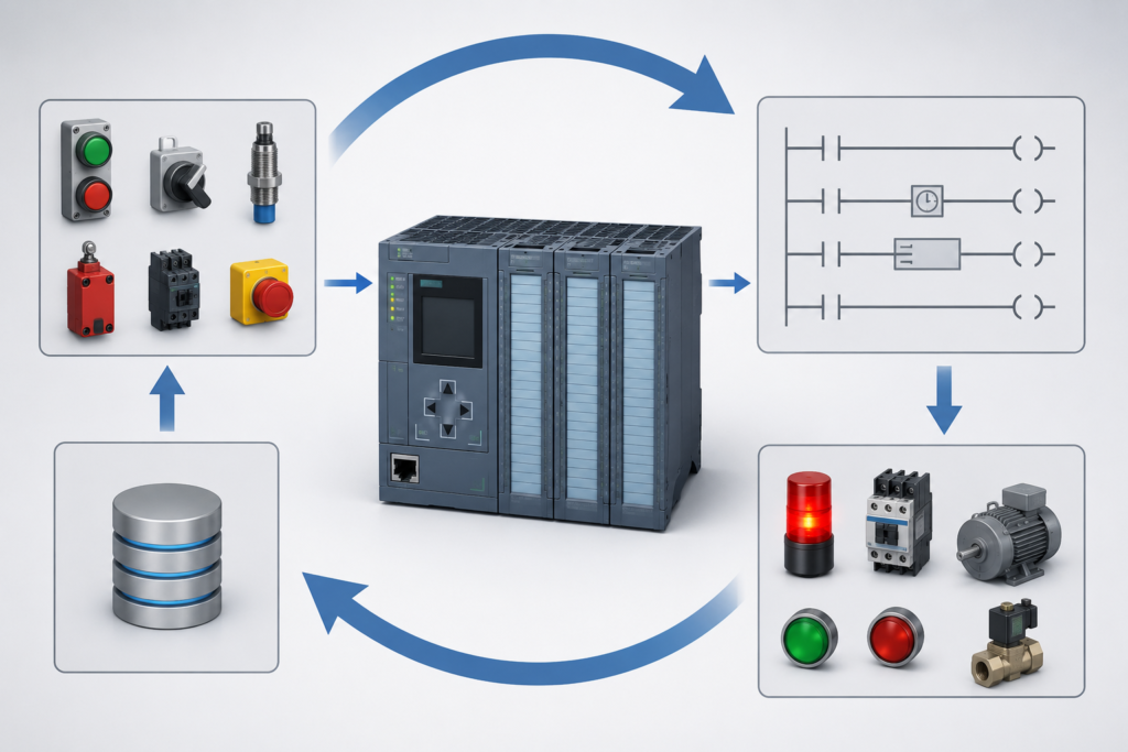
A PLC does not monitor every sensor, execute every instruction and update every output at exactly the same instant.
Instead, it performs these actions in a repeating sequence known as the PLC scan cycle.
A simplified cycle looks like this:
- Read the inputs
- Execute the control program
- Update the outputs
- Perform communication and diagnostic tasks
- Begin the next scan
This sequence may repeat thousands of times per second, but it is still divided into separate stages. That detail explains many strange problems seen during commissioning.
Step 1: Reading the Inputs
At the beginning of a typical scan, the PLC reads the states of its physical input modules.
Examples include:
- Push buttons
- Proximity sensors
- Limit switches
- Pressure switches
- Analog temperature signals
- Drive-ready contacts
The CPU usually copies these values into an internal memory area called the input process image.
The control program then works with this stored snapshot rather than continuously reading every input terminal.
Suppose a sensor changes state immediately after the PLC has finished reading its inputs. The program may not detect that change until the next scan.
For ordinary machine control, this delay is often too small to notice. For very short pulses or high-speed machinery, it can become significant.
Step 2: Executing the Program
After reading the inputs, the PLC begins executing the user program.
Instructions are normally processed in a defined order, such as:
- From top to bottom
- From left to right
- Block by block
- According to configured task priority
The PLC evaluates contacts, comparisons, timers, counters, calculations and function blocks using the input values available during that scan.
Program order matters.
For example, one network may set a motor command, while another network later in the program resets the same command. Even if both networks appear individually correct, the instruction executed last may determine the final state.
This is why assigning the same output or memory bit in several locations can produce confusing behaviour.
Step 3: Updating the Outputs
During program execution, the CPU usually writes output results into an internal output process image.
The physical outputs are then updated after the program finishes.
This means a digital output may not change at the exact moment its coil instruction becomes true in the program. The actual output terminal changes when the CPU reaches the output-update stage.
For example:
- A sensor is read at the start of the scan.
- The program detects the sensor.
- A motor-output command becomes true.
- The PLC completes the remaining program.
- The physical motor output is updated.
The total response time includes the input delay, program scan time and output-module delay.
Step 4: Communications and Diagnostics
The PLC must also handle activities that are not directly visible in ladder logic.
These may include:
- HMI communication
- PROFINET or PROFIBUS data exchange
- Remote I/O updates
- Drive communication
- Diagnostic processing
- Programming-device access
- Web-server requests
- System monitoring
These functions consume processing time and may operate at different update rates from the main control program.
An HMI, for example, may refresh a tag every 250 milliseconds while the PLC scans every 5 milliseconds. A value that becomes true for only one PLC scan may disappear long before the HMI requests its next update.
The operator may never see that signal, even though the PLC processed it correctly.
The PLC Then Repeats the Cycle
Once the scan is complete, the controller begins again.
Under stable operating conditions, the cycle appears almost continuous because it repeats so quickly.
However, the controller is still reacting to separate snapshots of the process. There are small timing gaps between:
- A field signal changing
- The input module detecting it
- The CPU reading it
- The control program responding
- The output module updating
- The HMI displaying the result
Most of the time, these delays are harmless. During commissioning, high-speed operation or intermittent faults, they can become extremely important.
PLC Scan Time Is Not Always Constant
A PLC may not take exactly the same amount of time to complete every scan.
Scan time can change because of:
- Conditional program branches
- Communication activity
- Complex calculations
- Loops and data processing
- Diagnostic events
- Large block calls
- Network interruptions
- Interrupt tasks
- Motion or technology functions
The CPU normally reports current, minimum and maximum cycle times. Monitoring these values can reveal whether the program occasionally becomes much slower than expected.
A program that normally scans in 4 milliseconds but occasionally reaches 40 milliseconds may miss events that appear reliable during normal testing.
Different Tasks Can Run at Different Rates
Modern PLCs may execute more than one program task.
For example:
- Main cyclic logic may run continuously.
- A timed interrupt may run every 10 milliseconds.
- A slower calculation task may run every second.
- A hardware interrupt may execute when an input event occurs.
Higher-priority tasks can interrupt lower-priority tasks.
This improves control performance, but it also creates the possibility that different parts of the program are working with data captured at different moments.
Shared data should therefore be handled carefully when multiple tasks can read or modify it.
Remote I/O Does Not Update Instantly
Remote input and output modules communicate with the PLC over an industrial network.
Their response time may depend on:
- Configured network update time
- Number of connected devices
- Network load
- Switches and topology
- Device processing time
- Communication faults or retries
A remote sensor may change in the field, but its new value must first reach the PLC through the network. The program then processes it, and the resulting output command may need to travel back across the network.
This total delay can be much longer than the CPU scan time alone.
Analog Inputs Add More Delay
Analog signals often include filtering to prevent noise from causing unstable readings.
A temperature, pressure or level input may therefore update more slowly than a digital input.
The delay can be influenced by:
- Sensor response time
- Transmitter damping
- Analog-module conversion time
- Configured interference suppression
- Software filtering
- Network update time
Increasing filtering creates a smoother value, but it also makes the signal respond more slowly to real process changes.
During troubleshooting, a delayed analog value can look like a slow PLC even when the CPU scan is perfectly normal.
Why Scan Behaviour Matters During Commissioning
Many timing problems remain invisible while the machine is operating slowly.
They appear when:
- Sensors activate close together
- Products move faster
- A valve responds more slowly than expected
- Network communication is interrupted
- An HMI command arrives between scans
- A signal remains active for only a few milliseconds
- Automatic and manual commands occur simultaneously
The program may work correctly during step-by-step testing but fail when the entire machine operates at production speed.
This is why commissioning should include realistic timing, rapid sequences and simultaneous conditions—not only individual input tests.
Troubleshooting Scan-Related Problems
When behaviour seems inconsistent, examine the timing chain.
Check:
- CPU cycle time
- Task execution periods
- Input filtering
- Remote I/O update rate
- HMI polling time
- Drive communication cycle
- Repeated writes to the same tag
- One-scan pulses
- Interrupt priorities
- Analog filtering
Trace functions are especially valuable because they record signals much faster than an HMI screen.
A watch table shows the current state. A trace shows what happened first, how long the signal remained active and which condition changed during the fault.
Final Thoughts
A PLC reacts quickly, but not continuously.
It reads a snapshot of the inputs, executes its instructions in a defined order, transfers the calculated output states and handles communication before repeating the process.
Once this behaviour is understood, many mysterious faults become easier to explain.
The problem may not be that the logic is wrong. The PLC may simply be reading, calculating or updating the signal at a different moment than the programmer expected.