Why PLC Logic Behaves Differently Under Load

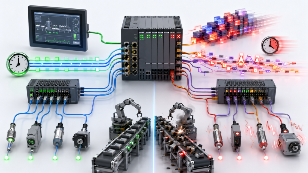
A PLC program may work perfectly during offline simulation and still behave differently when placed into a running industrial machine.

The code compiles. Every sequence step appears correct. Timers and interlocks operate as expected. Restart tests pass repeatedly.

Then production begins.

A motor occasionally starts late. A sequence stops for no obvious reason. Remote inputs arrive in a different order. An HMI button sometimes appears unresponsive. A startup that worked during testing suddenly becomes unreliable.

The logic itself may not be wrong.

The operating environment has changed.

Offline simulation provides controlled inputs and predictable timing. A live plant introduces network traffic, remote I/O delays, mechanical movement, operator actions and multiple events occurring at nearly the same time.

Offline Simulation Is an Ideal Environment

During offline testing, inputs are usually changed manually and one at a time.

The programmer may:

1. Turn on a start command.
2. Activate a permissive.
3. Simulate a sensor.
4. Confirm that the sequence advances.
5. Reset the program and repeat.

Every signal remains active long enough for the PLC logic to process it. There is no electrical noise, network jitter or mechanical uncertainty unless it is deliberately simulated.

The test environment usually excludes:

• Real field-device response times
• Industrial Ethernet traffic
• Remote I/O update intervals
• Sensor bounce
• VFD acceleration and deceleration
• Pneumatic valve delays
• Operator timing
• Communication interruptions
• Power-supply disturbances
• Simultaneous process events

Simulation proves that the logic works under the conditions included in the test. It does not prove that every live timing combination has been considered.

The PLC Has More Work During Production

A PLC running a real machine performs more than Boolean logic.

Depending on the system, it may also manage:

• PROFINET or EtherNet/IP communication
• Remote I/O stations
• HMI and SCADA requests
• Drive telegrams
• Modbus TCP devices
• Diagnostic processing
• Motion-control functions
• Safety communication
• Web-server access
• Data logging
• Recipe management
• Communication with other controllers

These activities consume processor time.

A program that scans in 3 milliseconds during a quiet test may take longer when the network, HMI and production devices are active.

The average scan time may still appear acceptable, while occasional peaks become much larger. Those brief peaks are often more important than the average value.

A fast sensor pulse that is reliably detected during a 3 ms scan may be missed during an occasional 20 ms cycle.

Communication Traffic Changes Timing

Industrial Ethernet is fast, but it does not make every device update at exactly the same moment.

Each device can have its own communication rate.

For example:

• A local digital input may update every PLC scan.
• A PROFINET station may update every 4 ms.
• A VFD telegram may update every 8 ms.
• A Modbus TCP device may be polled every 250 ms.
• An HMI may refresh its tags every 500 ms.

The PLC therefore receives information captured at different moments.

During offline testing, related signals are often changed together. In a live installation, those same signals may reach the controller during different scans.

This can create temporary combinations that the programmer did not expect.

Remote I/O Creates Additional Delay

A remote sensor signal must pass through several stages before it affects the program:

1. The physical process changes.
2. The sensor reacts.
3. The input module detects the new state.
4. Input filtering may delay the transition.
5. The remote station prepares updated data.
6. The network transfers the data.
7. The PLC receives the update.
8. The program evaluates the signal.

If the resulting command controls a remote output, the instruction must then travel back through the network before the actuator responds.

The complete response time can be significantly longer than the CPU scan time alone.

This matters in fast sequences where the program expects several conditions to change within a narrow timing window.

Field Devices Are Asynchronous

Field devices do not wait for the PLC scan to begin.

A sensor can switch halfway through a scan. A drive can update its status word while the main program is executing. An HMI command can arrive immediately before or after the logic that uses it.

These events occur independently.

The PLC handles them according to its configured task structure, communication cycle and process-image updates.

A live system may therefore process:

• A new sensor value with an old drive status
• A new command with an old permissive
• A recovered communication bit with stale process data
• A local input before a related remote input arrives

The values are not necessarily incorrect. They were simply captured at different times.

Production Creates Real Race Conditions

A race condition occurs when the outcome depends on which event reaches the logic first.

Consider two sensors used during startup:

• Sensor A confirms that a guard is closed.
• Sensor B confirms that a pneumatic clamp is home.

During offline testing, both conditions are switched on before the sequence starts.

In production, Sensor A may become true first. The program begins the startup sequence. Sensor B arrives one scan later, but the logic has already evaluated the missing condition and generated a fault.

On the next attempt, Sensor B happens to update first and the machine starts correctly.

The code has not changed. The execution timing has.

Race conditions commonly appear during:

• Machine startup
• Restart after an emergency stop
• Recovery after power failure
• Communication reconnection
• Fast product transfers
• Automatic-to-manual transitions
• Simultaneous reset and fault conditions
• Online program changes

Mechanical Equipment Is Not Perfectly Repeatable

Offline simulations tend to use ideal transitions.

A cylinder is either retracted or extended. A motor is either stopped or running. A valve changes state immediately.

Real equipment is less tidy.

A cylinder may take 450 ms during one cycle and 620 ms during another. A valve may react more slowly when cold. A conveyor may take longer to stop with a heavier product. A drive may need extra time to establish torque.

These variations can expose assumptions hidden inside the program.

A timer that allowed 500 ms for a cylinder may pass most tests and fail intermittently during production. The problem looks random, but the timing margin was simply too small.

Control logic should reflect realistic worst-case response times rather than ideal commissioning measurements.

Operator Interaction Is Difficult to Simulate

Operators press buttons at inconvenient moments.

They may:

• Press START twice
• Press START and STOP nearly together
• Change operating mode during a sequence
• Reset a fault before the original condition disappears
• Hold a button longer than expected
• Open a guard during recovery
• Issue an HMI command while communication is delayed

Offline testing is often performed slowly and deliberately by the programmer. Production operators do not follow the same timing pattern.

The program should define clear priorities for conflicting commands.

Typical rules include:

• Stop overrides start.
• Safety loss overrides all operating commands.
• An active fault overrides reset.
• Manual mode changes are accepted only in a safe state.
• A command is ignored until the previous transition is complete.

Without explicit priority rules, the outcome may depend on program order.

HMI Behaviour Can Hide the Real Problem

The HMI usually refreshes much more slowly than the PLC program.

A PLC may execute every 5 ms while the HMI polls a tag every 500 ms.

During one HMI refresh period, the PLC may complete 100 scans.

A permissive can disappear, stop a motor and return before the HMI reads it. The operator sees a healthy green indication and concludes that the motor stopped without cause.

Likewise, an HMI trend may appear stable while the PLC value is oscillating rapidly between updates.

For timing-related faults, use PLC traces, event latches and sequence histories rather than relying only on the operator screen.

Analog Processing Adds Hidden Dead Time

Analog signals often include several layers of delay:

• Sensor response time
• Transmitter damping
• Module integration
• Software filtering
• Network transmission
• PID processing
• HMI averaging

A filtered temperature or pressure value may look stable while the physical process has already changed.

Under production load, this delayed feedback can cause:

• Startup overshoot
• Late interlock operation
• Sluggish control response
• Oscillation
• Delayed shutdown
• Incorrect sequence transitions

Filtering should remove noise without making the real process invisible.

Online Edits Can Change Execution Behaviour

An online program modification may affect more than the edited instruction.

The change can alter:

• Block execution order
• Task duration
• Temporary states
• Timer conditions
• Retained values
• Communication loading
• Sequence initialization

A modification that appears harmless can create a short transitional condition while the process is running.

Changes involving sequence states, interlocks or shared data should be applied carefully. In some cases, a controlled stop and restart is safer than editing live production logic.

Common Symptoms Under Live Load

Intermittent startup faults

A permissive or remote-ready signal arrives later than expected.

Different result on each restart

Devices initialize at different speeds after power is restored.

Sequence skips or enters the wrong step

Inputs update asynchronously or multiple transitions are valid at once.

HMI command appears ignored

The command exists briefly, arrives between scans or is overwritten by another condition.

Motor starts or stops late

Network delay, task loading or output update timing adds response time.

Fault cannot be reproduced manually

Manual testing changes signals too slowly and removes the timing condition that causes the fault.

Program works when production is slowed

The extra time allows sensors, networks and actuators to complete their transitions before the logic evaluates them.

Measure the Real Scan Behaviour

Do not judge performance only from the current scan time.

Check:

• Current cycle time
• Minimum cycle time
• Maximum cycle time
• Task execution periods
• Task-overrun diagnostics
• Interrupt frequency
• Communication load
• Network update times
• HMI polling rates

A large maximum scan time can explain a fault even when the average value looks normal.

Also determine whether the program depends on one-scan pulses. A signal lasting one scan may become unreliable when task duration changes.

Trace the Entire Signal Chain

When a fault appears only under production load, record the sequence of events.

Capture:

• Raw field input
• Process-image input
• Filtered or processed input
• Communication status
• Current sequence step
• Transition condition
• Permissive result
• Output command
• Remote output state
• Device feedback
• CPU scan time

The objective is to identify what changed first and which state the PLC processed.

A watch table shows what is happening now. A trace shows what happened during the fault.

Design Logic for Real Plant Conditions

Reliable PLC logic should not depend on ideal timing.

Useful design methods include:

Require stable permissives

Important startup conditions can be required to remain true for a short, defined period before operation begins.

Use handshakes

Controllers, robots and drives should exchange request, acknowledge and complete signals rather than relying on exact timing.

Allow realistic transition time

A machine state should distinguish between command issued, movement in progress, confirmation received and timeout.

Use one writer per command

Avoid setting and resetting the same output from multiple locations. Calculate the final command in one place with visible priorities.

Monitor communication validity

Do not continue trusting the last received value indefinitely after communication fails.

Latch short events

Store brief faults and transitions until they are acknowledged or recorded.

Test worst-case conditions

Commissioning should include high production speed, simultaneous events, delayed devices, communication interruptions and restart recovery.

Final Thoughts

PLC logic often behaves differently under load because offline testing and live production are not the same environment.

Simulation provides controlled timing, ideal transitions and predictable inputs. A real plant adds network congestion, remote I/O delay, mechanical variation, operator interaction and multiple asynchronous events.

The code may be logically correct while the timing assumptions around it are not.

When a program works offline but becomes unstable after deployment, do not immediately rewrite the entire sequence. Measure scan time, record network updates, trace the relevant signals and inspect how the logic handles transitions.

Sometimes the program did exactly what it was written to do.

The plant simply delivered the information in an order the programmer did not expect.