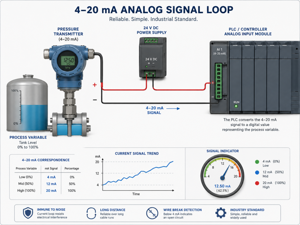
The 4–20 mA current loop remains one of the most widely used analog signal standards in industrial automation.
It is used to transmit measurements such as:
- Pressure
- Temperature
- Flow
- Tank level
- Valve position
- Speed
- Conductivity
- Process density
Compared with voltage signals, a current loop is generally less sensitive to voltage drop and electrical interference over long cable runs. That makes it well suited to factories, water-treatment plants, process facilities and other electrically noisy environments.
However, a 4–20 mA signal is not automatically reliable.
Poor grounding, damaged shielding, incorrect wiring, unstable loop power and electromagnetic interference can all produce misleading values. The PLC may receive a believable engineering measurement even though the physical signal is noisy, drifting or partially failed.
How a 4–20 mA Signal Represents the Process
A standard loop assigns:
- 4 mA to the minimum process value
- 20 mA to the maximum process value
For example, a pressure transmitter may be configured as:
- 4 mA = 0 bar
- 20 mA = 10 bar
The usable span is 16 mA.
At 12 mA, the signal is halfway between 4 and 20 mA:
(12 mA − 4 mA) ÷ 16 mA = 0.5The pressure is therefore halfway through the 0–10 bar range:
0.5 × 10 bar = 5 barThe PLC should display approximately 5 bar, assuming that the transmitter, analog module and scaling configuration all agree.
Why the Signal Starts at 4 mA
The 4 mA lower limit is known as a live zero.
If zero process pressure were represented by 0 mA, the PLC could not easily distinguish between:
- A genuine zero measurement
- A broken wire
- Loss of transmitter power
- A disconnected instrument
- An open current loop
With a live zero:
- Approximately 4 mA can represent a valid minimum process value.
- A current close to 0 mA usually indicates an electrical problem.
Many transmitters can also drive the output below or above the normal measuring range when they detect an internal fault. The exact alarm-current levels depend on the transmitter manufacturer and its configuration.
The PLC program should not assume that every current below 4 mA is simply a negative process value.
The Complete Current-Loop Path
A typical 4–20 mA measurement passes through:
- The physical process
- The sensor element
- The transmitter electronics
- The current loop
- Field cabling
- Terminal blocks and isolators
- The PLC analog input module
- Raw-value conversion
- Scaling logic
- Filtering
- PLC control logic
- HMI display
A failure anywhere in this chain can produce an incorrect final value.
The HMI does not display pressure directly. It displays a calculated number derived from the current received by the PLC.
Active and Passive Devices
One common source of wiring mistakes is misunderstanding whether the transmitter and analog input are active or passive.
A two-wire transmitter usually obtains its operating power from the current loop. A typical circuit may include:
24 V DC supply
→ transmitter
→ PLC analog input
→ 0 V return
Other devices may provide their own powered output.
The analog input may also be configured as:
- Active input
- Passive input
- Two-wire transmitter input
- Four-wire transmitter input
Connecting two active devices together or failing to provide loop power can result in:
- No current
- Incorrect current
- Diagnostic faults
- Possible equipment damage
Always check the wiring diagram for the exact transmitter and PLC module.
Loop Resistance and Voltage Burden
A current transmitter needs enough supply voltage to push the required current through the complete loop.
The loop may contain:
- Long cable resistance
- PLC input resistance
- Signal isolators
- Barriers
- Indicators
- Test points
- Terminal resistance
If the total voltage burden becomes too high, the transmitter may be unable to reach 20 mA.
The PLC may then display a value that stops increasing before the process reaches its true maximum.
For example, a transmitter measuring increasing pressure may rise normally until 17.8 mA and then remain there because insufficient voltage is available across the transmitter.
This can look like process saturation or incorrect scaling when the real issue is loop compliance voltage.
Electrical Noise
Current loops resist noise better than voltage signals, but they are not immune to interference.
Common noise sources include:
- VFD output cables
- Servo drives
- Large motors
- Contactors
- Solenoid valves
- Welding equipment
- High-current busbars
- Poorly suppressed relay coils
- Switching power supplies
Noise can produce:
- Rapid oscillation
- Random spikes
- Periodic disturbance
- Brief alarm activation
- Unstable PID control
- Nuisance interlocks
A useful clue is that the analog value changes when a particular motor or contactor operates.
Record the raw input while switching suspected equipment. If the noise begins at the same moment, inspect cable routing, shielding and grounding.
Shielding Problems
Shielded instrumentation cable helps prevent external electromagnetic fields from coupling into the signal conductors.
Problems occur when the shield is:
- Not connected
- Connected incorrectly
- Damaged
- Used as a current-carrying conductor
- Grounded at inappropriate locations
- Terminated with a long unshielded tail
- Routed beside VFD motor cables
The correct shield arrangement depends on the installation, equipment and grounding design.
In many systems, the cable shield is connected to protective earth at a designated point. However, blindly applying one grounding method to every system can create ground loops or EMC problems.
Follow the transmitter, module and site grounding documentation.
Ground Loops
A ground loop can form when parts of the analog system are referenced to ground through more than one path.
Small voltage differences between grounding points can create unwanted current and measurement error.
Symptoms may include:
- Slow value drift
- Offset that changes when machinery operates
- Unstable readings between buildings
- Different readings when a laptop or test instrument is connected
- Noise associated with VFD operation
- Correct current measurement but incorrect PLC value
Possible solutions include:
- Galvanic signal isolation
- Isolated analog input channels
- Improved equipotential bonding
- Correct shield termination
- Removal of unintended ground connections
- Isolated transmitter power supplies
Grounding changes should be planned carefully. Disconnecting a shield because it appears to reduce noise may create a larger susceptibility problem elsewhere.
Long Cable Runs
A correctly designed current loop can operate over long distances, but cable condition still matters.
Long runs introduce:
- Additional resistance
- Greater exposure to electromagnetic interference
- More terminal connections
- Increased lightning and surge exposure
- More opportunities for insulation damage
Inspect long field circuits for:
- Water ingress
- Damaged junction boxes
- Corroded terminals
- Incorrect splices
- Shared cables with power conductors
- Poor surge protection
- Insulation leakage
An insulation fault may not fully break the loop. It can instead create a drifting or unstable measurement.
Broken Loop or Open Circuit
A completely open circuit often produces a current near 0 mA.
Possible causes include:
- Broken conductor
- Loose terminal
- Disconnected transmitter
- Blown loop fuse
- Failed power supply
- Damaged junction box
- Incorrect polarity
- Failed transmitter
The analog module may report:
- Underflow
- Wire break
- Channel fault
- Minimum raw count
- Invalid quality
The PLC program should use these diagnostics.
Simply scaling every raw value into engineering units can produce a misleading number, such as a large negative pressure, instead of a clear instrument fault.
Partial Wiring Faults
Not every wiring failure creates a complete open circuit.
A loose or corroded connection may create:
- Intermittent spikes
- Sudden drops
- Temperature-dependent drift
- Vibration-related faults
- Increasing loop resistance
- Unstable measurements during machine movement
The signal may behave normally while the cabinet is open and fail again after the machine resumes operation.
Inspect terminals physically and use controlled movement or vibration testing where safe and appropriate.
Incorrect PLC Input Configuration
The analog module must be configured for the actual signal.
Common mistakes include selecting:
- 0–20 mA instead of 4–20 mA
- Voltage input instead of current input
- Incorrect channel range
- Wrong two-wire or four-wire mode
- Incorrect interference-suppression frequency
- Excessive integration time
- Disabled diagnostics
An input configured for 0–20 mA may still display a smooth process value from a 4–20 mA transmitter, but the scaling will be wrong unless the program compensates correctly.
Always verify the hardware configuration and the scaling logic together.
Incorrect Scaling
A generic scaling calculation is:
Engineering value =
(Raw value − Raw minimum)
×
(Engineering maximum − Engineering minimum)
÷
(Raw maximum − Raw minimum)
+
Engineering minimum
The exact raw values depend on the PLC and analog module.
The programmer must know:
- Raw count at 4 mA
- Raw count at 20 mA
- Engineering minimum
- Engineering maximum
- Data type
- Underflow and overflow ranges
Common errors include:
- Using 0 as the raw minimum when the module represents 4 mA differently
- Entering the wrong transmitter range
- Scaling the signal twice
- Reversing engineering minimum and maximum
- Using outdated calibration data
- Mixing bar, kilopascals and pounds per square inch
- Losing decimal precision through integer calculations
A wrongly scaled value may still appear believable, which makes the fault particularly difficult to notice.
Test Scaling at Several Points
Do not validate an analog channel at only one value.
Use a calibrated loop source or process calibrator to test:
- 4 mA
- 8 mA
- 12 mA
- 16 mA
- 20 mA
For a 0–10 bar transmitter, the expected results are approximately:
| Current | Expected pressure |
|---|---|
| 4 mA | 0 bar |
| 8 mA | 2.5 bar |
| 12 mA | 5 bar |
| 16 mA | 7.5 bar |
| 20 mA | 10 bar |
Also test:
- Current below 4 mA
- Current above 20 mA
- Open-circuit behaviour
- Diagnostic response
This verifies both normal scaling and fault handling.
Random Spikes
Brief spikes can come from:
- EMI
- Loose terminals
- Poor shielding
- Faulty transmitter electronics
- Module faults
- Unstable loop power
- Networked data corruption
- Incorrect grounding
A spike may last only one PLC scan and never appear on the HMI.
Use a PLC trace to record:
- Raw analog value
- Scaled value
- Filtered value
- Module diagnostic state
- Nearby output commands
- Motor and VFD status
- Supply voltage
If the spike occurs whenever a contactor or VFD switches, investigate EMC and suppression before changing the PLC logic.
Slow Drift
A slowly changing measurement may be caused by the real process, but it can also indicate:
- Transmitter calibration drift
- Temperature effects
- Ground-reference changes
- Moisture in the cable
- Unstable power supply
- Sensor contamination
- Blocked pressure impulse lines
- Analogue-module offset
Compare the signal with an independent calibrated measurement.
Long-term trend comparison between redundant or related sensors can also reveal gradual drift.
Flatlined Values
A flat analog value does not always mean the process is stable.
Possible causes include:
- Broken loop
- Frozen transmitter
- Analog module freeze
- Communication failure
- Saturation at the configured range
- PLC tag no longer being updated
- Excessive filtering
- HMI display failure
A value may remain at its last valid number after communication stops.
The PLC should monitor more than the measurement itself:
Process_Value
Signal_Valid
Channel_Diagnostic
Last_Update_Time
Communication_Healthy
A plausible value should not be trusted indefinitely without evidence that it continues to update.
Signal Saturation
If the process exceeds the transmitter range, the current may remain near its maximum value.
For example:
- Transmitter range: 0–10 bar
- Real pressure: 14 bar
- Output remains around its configured upper limit
The HMI may show a stable 10 bar even though the actual pressure is substantially higher.
Likewise, a process below the lower configured range may remain at the minimum or fault-current level.
Alarm logic should distinguish between:
- Normal high process condition
- High overrange
- Module overflow
- Invalid signal
- Transmitter fault
Filtering Can Hide the Real Signal
Filtering is commonly added because the raw value looks noisy.
A moving average or low-pass filter can produce a clean trend, but it also delays the measurement.
For example:
- Real pressure falls rapidly.
- Raw current drops.
- Filtered value decreases slowly.
- The low-pressure interlock remains healthy.
- The pump continues operating.
- The filtered value eventually reaches the trip point.
The shutdown logic may be perfectly correct. The data reaching it is simply late.
Filtering should remove noise, not hide real process changes.
During commissioning, compare:
- Raw current or raw PLC count
- Scaled value
- Filtered value
- HMI value
- Interlock state
Record all of them on the same timeline.
Separate Raw, Control and Display Values
One analog value does not need to serve every purpose.
A practical structure might include:
Pressure_Raw
Pressure_Scaled
Pressure_Control
Pressure_Display
Pressure_Valid
Possible uses:
- Raw value for electrical diagnostics
- Scaled value for engineering verification
- Lightly filtered value for interlocks
- Appropriately filtered value for PID control
- Smoother value for HMI display
This structure prevents heavy display filtering from delaying critical logic.
Measuring the Loop Correctly
When troubleshooting, measure the loop current using an appropriate calibrated instrument and safe procedure.
Common methods include:
- Opening the loop and connecting an ammeter in series
- Using a dedicated test terminal
- Using a loop calibrator
- Measuring across a known precision resistor
- Using a suitable clamp meter designed for low DC current
Avoid disconnecting a live process signal without understanding what the PLC and equipment will do when the loop opens.
The loss of one analog input may stop machinery, close valves or activate alarms.
Compare Three Values
For efficient troubleshooting, compare:
- Actual physical process value
Measured with an independent instrument. - Actual loop current
Measured electrically. - PLC engineering value
Observed from the raw and scaled PLC tags.
The comparison identifies the likely fault area:
- Physical value wrong and current agrees: process or instrument issue
- Physical value correct but current wrong: transmitter or loop issue
- Current correct but raw PLC value wrong: module or wiring issue
- Raw value correct but engineering value wrong: scaling issue
- PLC value correct but HMI wrong: HMI configuration or communication issue
This approach is more effective than changing filters and scaling parameters at random.
Useful PLC Diagnostics
A well-designed analog function block should expose:
- Raw channel value
- Scaled engineering value
- Filtered value
- Signal-valid status
- Underflow
- Overflow
- Wire break
- Channel diagnostic
- Rate of change
- Last update time
- High and low alarms
- Sensor fault
- Maintenance warning
The HMI should clearly distinguish between:
- Valid zero measurement
- Broken loop
- Under-range process condition
- Transmitter fault
- Stale data
Displaying all failures as 0.0 bar is misleading.
A Practical Troubleshooting Workflow
When a 4–20 mA value behaves incorrectly:
- Verify the actual process using an independent instrument.
- Check the transmitter range and units.
- Measure the loop current.
- Confirm the loop power supply.
- Inspect polarity and terminal connections.
- Check cable shielding and grounding.
- Review routing near VFD and motor cables.
- Examine the PLC module configuration.
- Monitor the raw PLC value.
- Verify the scaling calculation.
- Compare raw and filtered response.
- Check module and communication diagnostics.
- Test several known current values.
- Confirm HMI scaling and tag mapping.
Do not begin by changing the PLC program unless the signal chain has first been verified.
Final Thoughts
The 4–20 mA loop is reliable, but it is not immune to industrial reality.
Poor shielding, grounding problems, damaged wiring, incorrect input configuration and bad scaling can all produce unstable or inaccurate measurements.
The greatest danger is not always an obvious broken signal.
It is a believable value that no longer represents the real process.
Treat every analog measurement as a complete chain:
Process → transmitter → current loop → analog module → scaling → filtering → PLC logic → HMI
The PLC can only control from the current it receives and the numbers calculated from it.
When those numbers are wrong, correct logic still produces the wrong response.