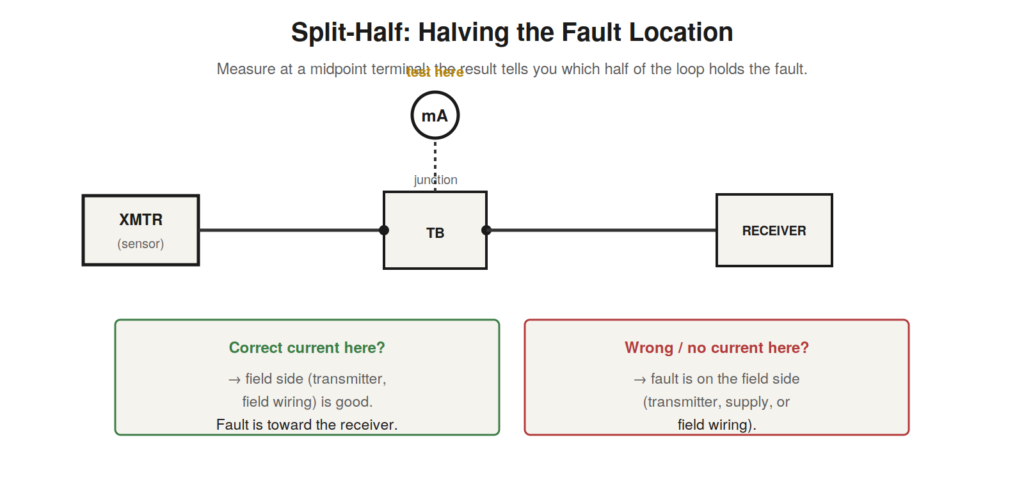
The split-half technique deserves a chapter of its own, because it is the single most efficient method for localizing a loop fault. Borrowed from the general principle of binary search, it finds a fault in a series loop with the fewest measurements by repeatedly halving the region that could contain it. Mastering it transforms loop troubleshooting from a sequential search into a rapid convergence.
How split-half works
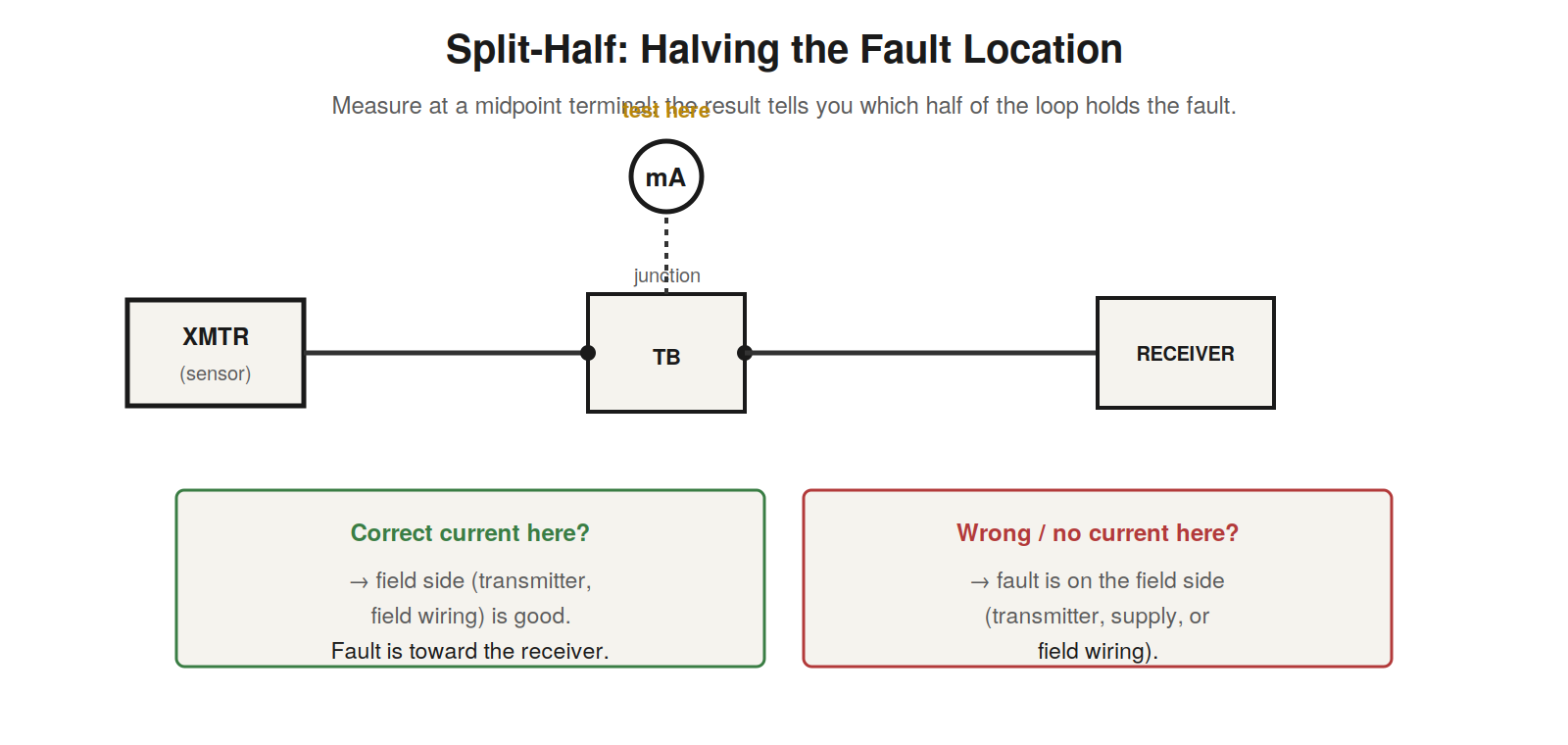
The split-half technique works by measuring the loop current at a point roughly in the middle of the loop — typically an accessible junction terminal — and using the result to eliminate half the loop. If the correct current is present at the midpoint, then everything from the transmitter to that point is working, so the fault must lie between the midpoint and the receiver. If the current is wrong or absent at the midpoint, the fault lies between the transmitter and the midpoint. Either way, one measurement has eliminated half the loop. You then repeat the process on the remaining half, measuring at its midpoint to halve it again, and continue until the fault is localized to a small section or specific element. This repeated halving finds the fault in far fewer measurements than checking each part in sequence, because each measurement cuts the remaining possibilities in half rather than eliminating just one.
Why it is so efficient
The efficiency of split-half comes from the mathematics of halving. Checking a loop element by element, you might need many measurements in the worst case, testing each section until you find the fault. With split-half, each measurement halves the region, so even a loop with many sections is narrowed down in just a few measurements — the number of halvings needed to isolate one section. This is dramatically fewer than a sequential search for a loop of any size. The technique’s power grows with the size of the loop: the more sections and access points a loop has, the greater the advantage of halving over sequential checking. For the long, multi-junction loops common in plants, split-half can localize a fault in a handful of measurements that would take many more to find by checking each section in turn. This efficiency is why split-half is the technique of choice for localizing loop faults, especially in larger installations where sequential checking would be slow.
Applying split-half in practice
Applying split-half in practice means using the loop diagram to identify the accessible measurement points — the junction terminals where you can read the loop current — and choosing ones near the middle of the remaining suspect region. The loop diagram shows where the junctions are and what is on each side, so you can pick a midpoint and know what the result implies. At each chosen point, you read the current (in series or across a sense resistor as appropriate) and compare it to what it should be, then eliminate the half that is confirmed good. Practical considerations include the availability of access points (you can only measure where the loop is accessible) and the invasiveness of the measurement (series measurement breaks the loop). But the principle is constant: measure near the middle, eliminate the good half, repeat. Combined with the fault-signature reading that starts the diagnosis and the isolation and injection that finish it, split-half provides the efficient localization step that makes the whole troubleshooting method fast, turning a potentially long search into a few well-chosen measurements that converge on the fault.
A worked split-half on a long loop
Consider a long loop with eight accessible junction points between transmitter and receiver, and a fault somewhere along it. Checking each junction in sequence from the transmitter might take up to eight measurements to find the fault. With split-half, you measure at the fourth junction first: if the current is correct there, the fault is in the second half (junctions five to eight), so you next measure at junction six, halving again; if correct there, the fault is at seven or eight, and one more measurement finds it — three measurements total. If instead the current was wrong at junction four, the fault is in the first half, and you halve that, and so on. In every case, three or four measurements localize the fault among eight sections, versus up to eight for sequential checking. On a loop with even more access points the advantage grows: doubling the number of sections adds only one measurement to the split-half search. This worked example shows concretely why split-half is so efficient — the halving finds the fault in a number of steps that grows only slowly with loop size, unlike sequential checking that grows in direct proportion.
Split-half beyond wiring: the whole loop
Split-half applies not just to locating a break in the wiring but to dividing the whole loop into its major elements — transmitter, wiring, receiver — which is a useful way to think about it. The first, biggest split is often conceptual: is the fault on the field side (transmitter and field wiring) or the control-room side (receiver and its wiring)? Measuring the current at a junction between field and control room answers this, halving the loop into its two major parts. From there, split-half continues within the identified part: within the field side, is it the transmitter or its wiring; within the control-room side, is it the receiver or the scaling. Each split narrows down which element holds the fault. Thinking of split-half at this level — dividing the loop into transmitter, wiring, and receiver, and determining which contains the fault — complements its use for locating a specific break, and it structures the whole diagnosis. The technique’s principle, halving the region of uncertainty, works at every scale from ‘which major element’ down to ‘which section of wire,’ and applying it at each level drives the diagnosis efficiently from the whole loop to the specific fault.
When access points limit the splits
Split-half is ideal in principle, but in practice the available access points limit where you can split, and adapting to this is part of applying the technique. You can only measure the loop where it is accessible — at junction terminals, marshalling points, and the like — so the splits happen at these points rather than at any arbitrary midpoint. If access points are sparse, the splits are coarser, and if they are plentiful, the splits can be finer. Reading the loop diagram to identify the accessible points, and choosing the one nearest the middle of the remaining suspect region, applies split-half as well as the access allows. Where access is limited, the technique still helps — each available split still halves the region among the accessible divisions — but the localization is only as fine as the access points permit, after which other methods (isolation, injection, inspection) take over for the final identification within the smallest accessible section. Understanding that access points constrain the splits keeps expectations realistic and guides the practical application: use the accessible points to halve the region as far as possible, then switch to element-level isolation for the final step. Split-half localizes to the smallest section the access allows, and the remaining methods finish within it.
A general principle worth knowing
Split-half is a specific instance of a general problem-solving principle — binary search, or divide and conquer — that is worth recognizing because it applies far beyond loops. The principle is that to find something in an ordered or connected space, repeatedly halving the space is far more efficient than searching linearly. It applies to finding a fault in a series loop (split-half), a break in a cable (test the midpoint), a problem in a sequence of stages (check the middle stage), and countless other search problems. Recognizing split-half as this general principle both deepens your understanding of why it works and lets you apply the same thinking to other problems. Whenever you must locate something in a connected chain — electrical, mechanical, logical — the divide-and-conquer principle of testing the middle and eliminating half applies, and it is always more efficient than checking each element in turn. Split-half in loop troubleshooting is one application of this powerful general principle, and understanding it as such — not just a loop trick but an instance of divide and conquer — enriches both your loop troubleshooting and your general problem-solving, since the same halving logic speeds the search for a fault in any connected system, not only current loops.
Split-half combined with the signature
Split-half works best combined with the fault signature, because the signature guides where to start splitting and what to expect at each split. The signature tells you the fault class, which suggests where the fault is likely to be, informing your first split. For a dead loop (0 mA), you split to find where the current disappears, expecting 0 mA on the faulty side. For a wrong-value loop with a healthy current, split-half of the loop may not even be needed — the signature already points to scaling rather than a loop break. For an erratic loop, split-half can localize an intermittent connection by finding where the erratic behavior originates. So the signature and split-half work together: the signature classifies the fault and suggests the approach, and split-half localizes it where localization is needed, with the signature informing what each split should show. Using them together — signature first to classify and guide, split-half to localize — is more effective than either alone, because the signature focuses the split-half search and interprets its results. This combination reflects the whole method’s integration: read the signature to understand the fault, then apply the appropriate localization, with split-half as the key localization tool guided by what the signature revealed. Signature and split-half are partners in efficient loop diagnosis.
Mastering split-half pays off everywhere
Mastering the split-half technique pays off across all your loop troubleshooting, because localizing a fault is a step in nearly every diagnosis, and split-half is the efficient way to do it. Whenever a fault must be located in a loop — which is most faults — split-half finds it in the fewest measurements, so mastering it makes every such diagnosis faster. The technique is simple in principle but takes practice to apply well — choosing good split points, interpreting results, adapting to available access — and mastering it means these become fluent. A technician who has mastered split-half localizes faults quickly and confidently, while one who checks loops sequentially is slower. Given how often fault localization arises, mastering split-half is a high-value investment, repaying itself on every fault that must be located. It is worth practicing deliberately — applying it on real loops until the choice of split points and interpretation of results is second nature — because the payoff, faster localization on nearly every diagnosis, is large and continual. Split-half is the key localization technique, localization is central to troubleshooting, and mastering split-half therefore accelerates the core of loop diagnosis. The effort to master it — to apply the halving efficiently and adaptively — pays off everywhere loops must be diagnosed, which is why it deserves the deliberate practice to make it a fluent, reliable tool.